Bin Matrix Dialog

This dialog is opened when you select the Convert to Matrix -> 2D Binning... command from the Convert to Matrix menu. It allows to customize the process of generating a new matrix by counting the number the data points falling within a given XY range and storing the bin counts as Z values in this new matrix.

The initial coordinates of the output matrix are automatically calculated from the input data range, but of course you can customize them via the input boxes from the Matrix Coordinates group box. The Columns and Rows input boxes in the Matrix Dimensions group allow to specify the number of bins in the X and respectively Y range.

A 2D color map preview of the result matrix is displayed on the right side of the dialog, the color scale being connected to the number of data points in each bin.

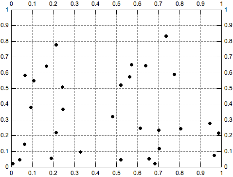
In order to understand how the frequency count process works please consider the following example: the table to be converted has two columns (X and Y) both containing random values between 0 and 1. We decide to create a new matrix with 10 rows and 10 columns, that is 100 bins. If we represent the input data using a scatter plot we get the graph bellow, where the scale divisions were changed to have a 0.1 step for both axes. In this graph, each square of the plot grid represents a 2D bin. QtiPlot counts the number of scatter points in each square and stores these values in the new matrix.

If the option Create Plot is checked, QtiPlot automatically shows a 2D color map plot or a 3D bars plot of the result matrix when the OK button is pressed.

When the option Auto is selected in the Recalculate box, QtiPlot also creates a connection between the source data table and the resulting matrix, so that every time the values in the table are modified the matrix window is automatically updated. The connection can be disabled at any time via the Matrix Properties dialog.